[Day 130] CS109: MAP, Naive Bayes, Logistic Regression
Hello :)
Today is 130!
A quick summary of today:- covered Lecture 22: MAP, Lecture 23: Naive Bayes, Lecture 24: Logistic Regression from Stanford's CS109
From 11pm later, to 3am (I believe) is the 3rd day of MLx Fundamentals, and I will share about the 2 sessions tomorrow.
Lecture 22: MAP
We saw new method for optimization: gradient descent (or ascent for now).


Probabilities are beliefs, and incorporating prior beliefs is useful.
MAP - allows us to incorporate priors for param estimation.
 Instead of choosing params that maximise the likelihood of the data, MAP (the Bayesian approach) gives us the params that are most likely given the data.

 MAP helps to not overfit. However, MLE works for more than just estimating p.

How can we generalize MAP (and maybe do it ourselves too)?
 (the normalization term is a constant so it can go away)

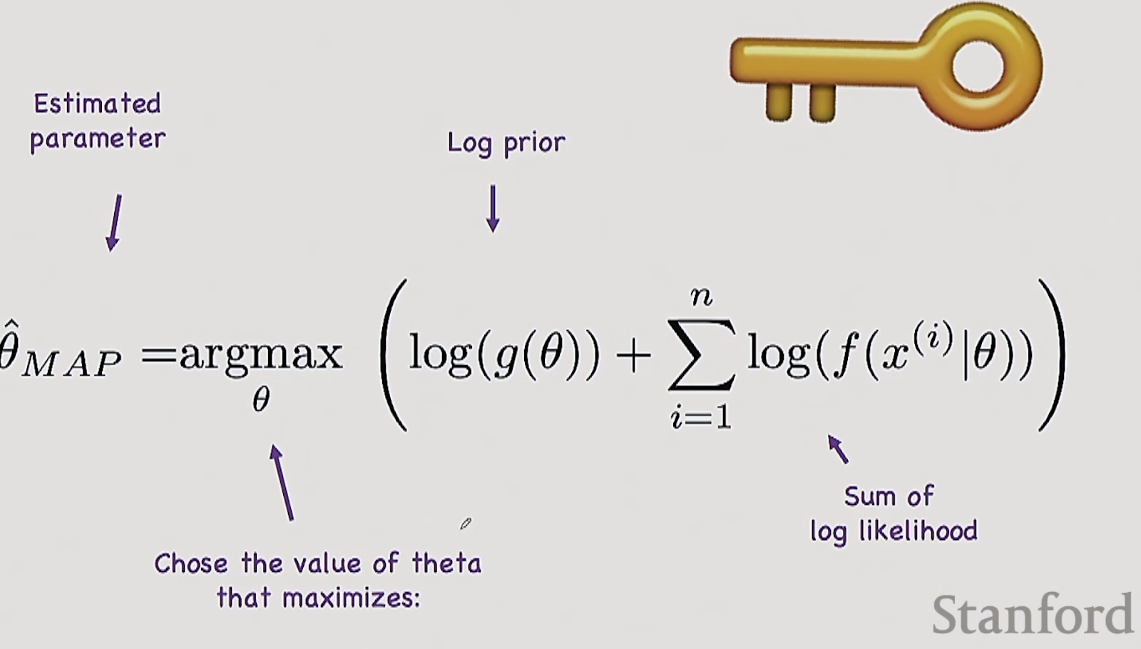
Doing MAP for Pareto alpha ~ N(2, 3)
 If we look at the bottom, if we put alpha = 2, that will make the prior term 0, but if we put a alpha larger than 2, i.e. 3 (larger than the mean of our prior belief), that term will end up a negative number, ths gradient will pull us closer to 2. And if we put an alpha that’s smaller than 2, it will pull us closer to 2 again but from the other direction.

we are done with the 1st part. :party:
Lecture 23: Naive Bayes

 What are the params that we need to learn?
 6 in this classification case (there is a bit of redundancy here (if we know Y=0 is theta5, then we know Y=1 is 1-theta5))
How do we estimate these probabilities?
 MLE says: just count
MAP says: count and add imaginary trials The probs dont add to 1? We got rid of the normalization constant!
So the result is y=1. m=3 ? same thing
 m=100? Same thing. Thats a lot of params.
Big O is 2^m!!! Brute force Bayes lets us down. But that assumption is not great. x2 might totally depend on x1 for cases like Kung Fu panda 2 and Kung Fu panda 1.


How to evaluate a Naive Bayes classifier?

Lecture 24: Logistic Regression
How can we generalize MAP (and maybe do it ourselves too)?
Doing MAP for Pareto
we are done with the 1st part. :party:
Lecture 23: Naive Bayes
Firstly, lets see brute force Bayes
How do we estimate these probabilities?
MAP says: count and add imaginary trials
we can use the Laplace prior - which is adding 1 imaginary trial for each outcome
Imagine we have got the probs with MAP now, and a test user comes.
So the result is y=1.
The above case was when m=1, we have 1 feature. Now, for m=2
Big O is 2^m!!! Brute force Bayes lets us down.
Calculating that P(x|y) is too expensive. Instead, lets assume that every xi is independent, so ~
How to evaluate a Naive Bayes classifier?
Lecture 24: Logistic Regression
Important notations:


 It takes the inputs and predict whether or not Y = 1. So you want the prob that Y = 1 given your inputs. It takes all the inputs, each goes through this step where it gets weighted by params and each channel gets summed into z, which then is squashed to get a probability with sigmoid.
Why is there x0 ? People found that if we include an offset, the model works better, to simplify we set x0 = 1.

 How does that look in code?

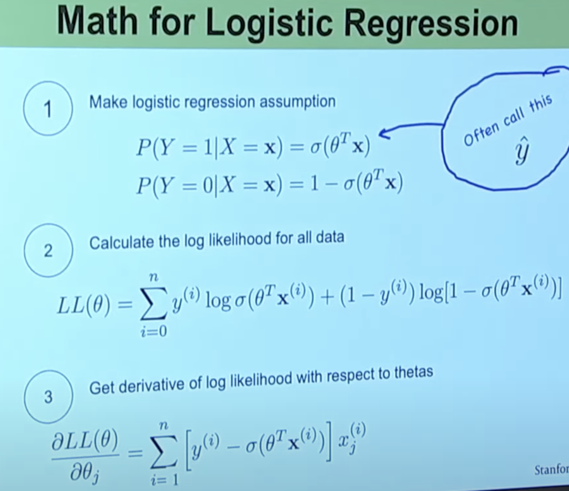
 There is something beautiful about sigmoid - its derivative is sigmoid multiplied by 1 - sigmoid


In classification we care about P(Y|X).
In Naive Bayes we can do that, but we make the dangerous assumption of independence. Can we model P(Y|X) directly? Yes - *logistic regression enters the room*
Logistic regression gives us a machine that’s got some params in it (that are movable), you will choose great values for the params such that your machine when it takes in Xs, just outputs things that are close to the prob that Y = 1 (or 0 for the opposite case).Why is there x0 ? People found that if we include an offset, the model works better, to simplify we set x0 = 1.
That is all for today. There is only a few lectures left which is a bit sad :( Professor Chris Piech is so amazing.
That is all for today!
See you tomorrow :)

