[Day 57] Stanford CS224N - Lecture 1. Word vectors

 Hello :)
Today is Day 57!

Quick summary of today:

• Got introduced to word vectors with lecture 1 + small showcase

• Read the paper and took notes about:

• Efficient Estimation of Word Representations in Vector Space (word2vec)

• Distributed Representations of Words and Phrases and their Compositionality (negative sampling)

First I watched the lecture by Professor Manning, and then I read the papers so some of the material was overlapping, but there were still interesting new parts in each of the three. 

1) Lecture notes

My notes from the lecture were not that long so I will first share them.

After the lecture, there was a small colab document I could run through. 

In the lecture, we mention about matrix multiplication and the larger the dot product between the 2 words, the more similar they are -> exp(u0T @ vc)

So in the colab there was a model loaded.

And I searched for the word embeddings of bread and baguette which in my view are similar words. 

In the below pic, if a 2 values from both matrixes are both positive, or both negative, that means the output of the matrix mul for that specific value will be positive, which overall means, more similar.

To find it easier to see, I used this np.sign to see how similar they are, and there are a de

Then I went to see what words are similar to bread according to the model:

And then. took flour and bread and saw that compared to break and baguette, their True values are more (which by itself is not a complete indicator of similarity, but still is can indicate some similarity)

Then in the word2vec paper, they proposed that with such word vectors we can do analogies by simple algebraic operations. I.e. start with a word like king, substract man from it, add woman and what word is the word that should be given? (queen)

And I had some fun with this too:

But as we can see if the words we are searching for did not exist in the model, or were very rare, then the output does not make sense. In the first one, hanbok is korea's traditional piece of clothing, but I have no idea what zenana is haha.

2) word2vec paper summary

1. Intro

Before word2vec, many nlp systems treated words as single units that do not have any notion of similarity. while this provided simplicity and robustness, such techniques had limits. for instance higher volume of data resulted in good performance, but if big data was not available, the models had limitations. Data was the limitation. but with the progress of ML, the newer and more complex models could be trained on larger data and outperform the simpler ones.

They used a, back then, recent technique for word representation that not only puts similar words closer to each other, but also words can have multiple degrees of similarity.

2. Popular neural network models

• Feedforward Neural Net Language Model (NNLM)

It consists of input, projection, hidden and output layers. At the input layer, N previous words are encoded using 1-of-V coding, V is the size of the vocab. After, the input layer is projected to a projection layer P that has dimensionality N × D. Also, since only N inputs are active at any given time composition of the projection layer is relatively cheap. However, it becomes complex for computation between the projection and the hidden layer, as values in the projection layer are dense.

• Recurrent Neural Net Language Model (RNNLM)

RNN based language models were proposed to overcome some of the limitations of the NNLM, such as the need to specify the context length, and because RNNs can theoretically represent more complex patterns than shallow NNs, and through a recurrent matrix, that forms like a short-term memory, info from the past is passed to the current input. 

3. New log-linear models

Previous models come with non-linear hidden layers, which complexify them. But the paper wants to look for a method that might not be able to represent data as precisely as NNs, but can be trained efficiently on much more data.

Furthermore, they propose 2 models.

• Continuous Bag-of-Words CBOW Model

Similar to the FF NNLM where the non-linear hidden layer is removed and the projection layer is shared with all words (not just the projection matrix), so all the words’ vectors are averaged. This model is called bag of words since the order of words in the history does not matter when it comes to the projection. In addition, they use words from the future. The paper mentions that they achieved the best results using a log-linear classifier with 4 future, 4 past words as the input, and the goal is to predict the middle word.

• Continuous Skip-gram Model

this one is similar to CBOW, but instead of predicting the middle word based on its context, it uses a word as the input to a log-linear classifier with continuous projection layer, and then predict its context. This method was found to be efficient when trying to predicted larger context, but with that the computational complexity rose.

4. Results

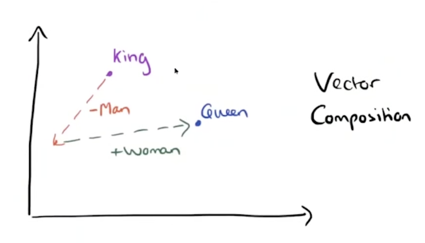
To show results, they proposed to use analogies, for example big is to bigger is as small is to ____? And they found that such questions can be answered with algebraic operations with the vector representation of words. 

X = vector(‘bigger’) - vector(‘big’) + vector(‘small’), then from the vector space a word that is closes to X (measured by cosine distance) is given as the answer. They evaluated the accuracy of the model and assumed a correct answer only if the closest word to the vector computed is exactly the same as the correct word in the question. For instance, if the model is given the pair (king, queen) the correct word that the model should predict as closest might be "queen”. (more pairs in the 1st pic below)

The results also compared the RNNLM, NNLM, CBOW and Skip-gram models. And amongst them the CBOW (bag of words model) did the best when it comes to syntactic accuracy with 64%, but it lacked in semantic accuracy and came in 2nd with 24%. Whereas the skip-gram model scored more than double compared to the 2nd and 3rd place modes when it comes to semantic accuracy, and it was 2nd in syntactic. 

3) negative sampling paper

1. Intro

Distributed representations of words in a vector space helps learning algorithms to achieve better performance in NLP tasks by grouping similar words. Compared to, back then, other models, the skip gram model we saw in the 1st paper, does not invlove matrix multiplication into its training process which makes that process very efficient and a singple machine implementation can train on more than 100 billion words in 1 day. In this paper, the researchers propose that subsampling of frequent words during training results in a significant speedup and improves accuracy of the representations of less frequent words. They also propose a simplified variant of Noise Constrastive Estimation (technique that involves distinguishing between true data and noise samples) for training the skip-gram model which comes with better results compared to the originally used hierarchical softmax.

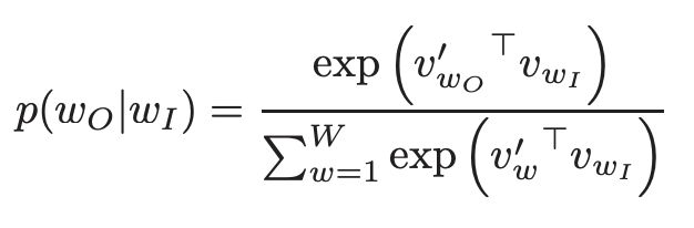
2. The skip-gram model

Its goal is to find word representations that are useful for predicting the context around a word/document. To achieve this, the model aims to max the avg log probability:

and the basic skip-gram defines p(Wt+j | Wt) with the softmax

But this formulation is impractical because the cost of computing delta log p(wo, wi) is proportional to W, which is often 10^5~10^7.

To overcome that, a computationally efficient approximation of the full softmax is called the hierarchical softmax. And its main advantage is that instead of evaluating W output nodes in the NN to obtain the probability distribution, it only needs to evaluate log2(W) nodes. 

3. Negative sampling

It is an alternative to the above is NCE which says that a good model should be able to differentiate data from noise by means of logistic regression. It works by randomly sampling a set of "negative" examples (words not within the context of the target) alongside positive examples (words that are within the context of the target) during training. 

4. Subsampling of frequent words

In a very large body of text, words like “the”, “a”, “in” can occur millions of times, and they provide less value compared to the rarer words. For example the words France and Paris are helpful to the skip-gram model, but the occurance of France and the togehter right next to each other will be most likely higher. To deal with this imbalance of words, they used a sub-samping approach where each word Wi in the training data is discarded with a probability:

where f(Wi) is the frequency of the word, and t is the chosen threshold.

5. Evaluation

To evaluate Hierarchical softmax (HS), Noise contrastive estimation (NCE), negative sampling (NGE) and subsampling of the training words, they used the same small:smaller = big: ? method as the word2vec paper. And the results are: 

6. Learning phrases

Many words cannot be explain just by learning the meaning of individual words - such as New York Times. To tackle this, they find words that appear frequantly together and infrrequentyl in other contexts, and such phrases are replaced by unique tokens. But cases like “this is” remains as is. After doing so, the analogy method was used again for evaluation. Results:

Looking forward to the next lecture tomorrow :)

That is all for today!

See you tomorrow :)