[Day 158] 50 minutes of audio in the Scottish dataset + exploring Mixture Density Networks in GNNs
Hello :)
Today is Day 158!
A quick summary of today:- created a better dataset preprocessing 'pipeline' for new audio files
- read a bit about Mixture density networks and their application
Firstly, about the Scottish dataset
The latest dataset has ~50 minutes worth of Glaswegian (Scottish) accent clips. Amazing ^^ [huggingface link]
I also finetuned microsoft's SpeechT5 on this latest data, but I am still getting a bit robotic outputs. I need to play more around with the trainer setup.
As for the 'pipeline' ~
It starts with renaming the audio files (so that we have some kind of tracking), I rename them by adding the preprocess date.

create_audio_metadata_csv(transcriptions_csv, filenames_df, audio_files_path, output_csv)
It takes a transcription csv that has 1 column with transcriptions, a 2nd csv with file names, path to the audio files, and where to output the csv which contains file_name, transcription, length_seconds, sampling_rate
Final is concatenating the old metadata csv with the new one (and also add some default info like gender, class, accent info)

As for the papers I read today at the lab
First, Estimating city-wide hourly bicycle flow using a hybrid LSTM MDN
I read this over the top for now, because I was interested in how they applied mixture density networks on an LSTM model
Simple LSTM


Introduction
The shared E-scooter service, integrating GPS, IoT, and API technologies, offers a convenient, flexible, and eco-friendly alternative to private vehicles for short trips, promoting public transportation usage and reducing carbon emissions. Its rapid growth in the U.S. necessitates real-time demand forecasting for efficient urban planning, fleet management, and maintenance to balance supply and demand effectively.
E-scooter demand prediction challenges
- spatial-temporal trip demands with extreme sparsity and imbalance
- difficult in predicting complexity and heterogeneity
- lack of a more systematic integration of the correlations between various factors and the expression of urban complexity
Contributions
- recluster spatial data and implement fusion loss functions with a loss penalty to mitigate trip demand accuracy deterioration due to demand sparsity and imbalance
- to simulate the relationship between urban complexity and shared e-scooter trip demands, different aspects are incorporated into the graph representation - i.e. built environments, weather conditions, periodic features
- building upon DCRNN a model that outperforms other benchmark models is proposed
Related work
Multivariate statistical analysis and regression for shared E-scooter usage correlation
Data-driven approaches analyzed correlations between ridership and various factors, including built environments, weather conditions, and periodic features, across different cities. Key findings include population density and education levels positively impacting E-scooter trips, city center proximity and high street density increasing ridership, and varying land use types influencing usage differently. Additionally, weather conditions significantly reduce trip frequency, and trip patterns vary between weekdays and holidays. Despite these insights, real-time accurate predictions for local subareas are still lacking, with deep learning models proposed as a potential solution.
Deep learning methods for shared E-scooter trip demand prediction
Traffic demand prediction has gained significant attention with the use of deep learning models, showing promising results. Key advancements include integrating spatial and temporal dependencies through combined models like RNNs and CNNs, with recent approaches leveraging graph convolutional networks for complex traffic networks (TGCN). For shared mobility, including E-scooters, models like CNN-LSTM, multi-graph convolutional, and gated graph convolutional networks have been developed to predict demand, considering dynamic origin-destination relationships and various influencing factors like built environments and weather conditions.
Methodology
Framework of trip demand prediction

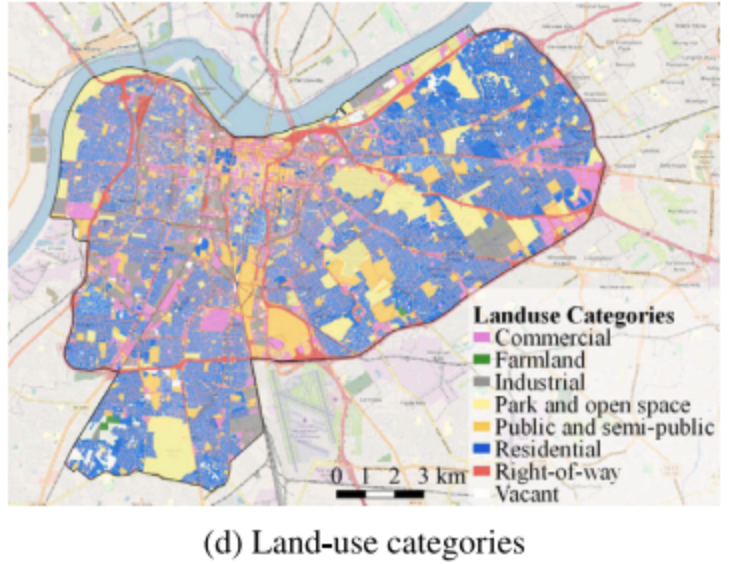
- Data collection - data include OD shared E-scooter trip data, population density, spatial relationships, POI, land use, and weather conditions in Louisville
- Spatial data reclustering - mapping data to geographical divisions
- Graph representation - the above are converted into comprehensive graph representations with graphs, nodes, and edges to capture the spatial-temporal dependencies for trip demand prediction
- Model training - a model specifically for sparse trip demand prediction is proposed, and training is adjusted
- Pick-up demand prediction - after fine-tuning the model, an optimal model is obtained that can predict the pick-up demand in the next hour in each region
- Universal features - weather and periodic features; apply time-series information, including year, month, week, and hour, as features and transform them into cyclical representations via cosine and sine functions based on their periodic behaviours
- Node features - extract the hourly pick-up demand as the first dimension feature, which is specified with negative integers to distinguish it from the drop-off demand as positive integers; by contrast, the hourly trip drop-off demand is the second dimension feature with positive integers. The sum of hourly trip pick-up and drop-off demands is the third dimension feature, which would be zero if rented and returned E-scooters share the same numbers. Other features representing urban built environments include spatial distance to the city centre, street density, intersection density, and population density for each region
- Edge features - the three spatial relationship between the origins and the destinations are distance, POI similarity, and difference in land-use entropy. POI similarity is calculated using Pearson's correlation coefficient to estimate functional similarity between two regions. Land-use entropy ranging from 0 to 1 is used to estimate the equilibrium between all available land uses for each region and calculate the differences between origins and destinations.
Model architecture
The introduced model is a modified version of DCRNN.

Data description
E-scooter data from Kentucky, USA. This research focuses on next hour pick-up demands as prediction targets.
- Shared e-scooter OD trip dataset

- population dataset

- street network and POI dataset

- land-use dataset
Strategies for the imbalanced data
- Spatial data reclustering: to integrate diverse learning features from different data sets measured across various standard divisions, data must be reaggregated and remapped into uniform geographical divisions. The study proposes reclustering prediction divisions from geographical census blocks to regions that better reflect the relationship between shared E-scooter trips and built environment factors. Using a hierarchical clustering method based on pick-up demand, the resulting reclustered regions, depicted in Fig. 5, highlight areas of higher demand, with low-demand regions being excluded from model training

- Fusion loss function and evaluation metrics: The proposed fusion loss function combines mean absolute error (MAE) and multi-classification loss with a penalty to address sparse and imbalanced data. It categorizes trip demand into different levels to improve performance and uses Jenks natural breaks algorithm to define six classes, later simplified into three levels for practical use. Evaluation metrics include MAE, RMSE, F1 score, and AUC, with the focal loss emphasizing minority samples and a loss penalty preventing the model from predicting zero demand excessively.

Experiments
Baselines
GCRN (with GRU and with LSTM), TGCN, A3T-GCN, 3 variants of the proposed model
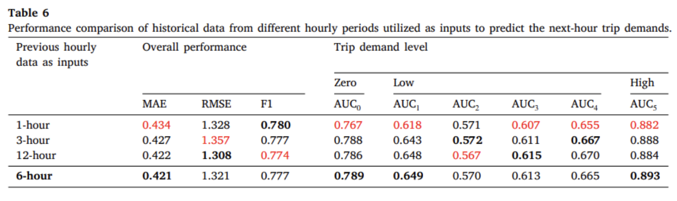
Average prediction performance over different periods

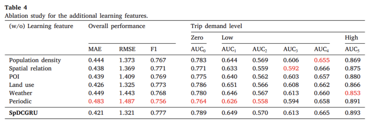
Ablation study for the additional learning features
Contribution of fusion loss

Overall
That is all for today!
See you tomorrow :)

