[Day 156] Final XCS224W: ML with Graphs homework

 Hello :)
Today is Day 156!

A quick summary of today:

• finished and submitted the last assignment of the Stanford XCS224W: ML with graphs course

• read a few more papers about spatial-temporal graph neural networks

As with the previous ones, I am not allowed to share anything related to the homework. All I will share is that I got the full score haha

As for the new papers I read today. 

I found about pytorch-geometric-temporal. It is an extension of the pytorch-geometric library that implements popular spatial-temporal GNN papers' architectures. 

I feel like I do not want this blog to be filled with posts on the same topic 5 out of 7 days of the week (at least that is how I feel right now as I am doing literature review on spatial-temporal GNNs' application in intelligent transportation systems), so I will try to do some extra studying after my lab and share it here. I will still share what I do in the lab and what I study there, but it will be just a part of a blog post, rather than the whole thing.

The reference graph is getting bigger and bigger, soon nodes might become to small to see.

Today I read the papers the implementation of which is in pytorch-geometric-temporal and I had not covered so far.

• Adaptive Graph Convolutional Recurrent Network for Traffic Forecasting

Introduction

The paper proposes two mechanisms that build upon the popular GCN

• A node adaptive parameter learning (NAPL) module, which learns node-specific patterns for each traffic series. NAPL factorises the parameters in traditional GCN and generated node-specific parameters from a weights pool and bias pool shared by all nodes according to the node embedding
• A data adaptive graph generation (DAGG) module, which infers the node embedding (attributes) from data and generates the graph during training.
• NAPL and DAGG are combined with recurrent networks and Adaptive Graph Convolutional Recurrent Network is proposed.

Experiments

Datasets

PeMSD4, PeMSD8

Baselines

HA, VAR, GRU-ED, DSANet, DCRNN, STGCN, ASTGCN, STSGCN

Metrics

RMSE, MAE, MAPE

Results

• Attention Based Spatial-Temporal Graph Convolutional Networks for Traffic Flow Forecasting

Introduction

ASTGCN consists of three independent components designed to model different temporal properties of traffic flows: recent, daily-periodic, and weekly-periodic dependencies. Each component has two main parts: 1) a spatial-temporal attention mechanism that effectively captures dynamic spatial-temporal correlations in traffic data, and 2) a spatial-temporal convolution that uses graph convolutions to capture spatial patterns and standard convolutions to describe temporal features. The outputs of these three components are then weighted and fused to produce the final prediction results.

Observations close to each other in space and time are dynamically correlated and to solve traffic problems, effectively extracting spatial-temporal correlations of traffic flows is essential.

In the figure, the darker the colour line is, the stronger the connection and influence on each other. Also depending on time, a location's influence varies as well.

CNN and GCN models still fail to capture the spatial-temporal features that come from dynamic traffic data, so the proposed method ASTGCN aims to collectively predict traffic flow at every location on the traffic network.

Attention based spatial-temporal GCN

The structure consists of three independent components with the same structure, which are designed to model recent, daily-periodic, and weekly-periodic dependencies of the historical data.

Suppose the current time is t0, and the size of the predicting window is T_p.

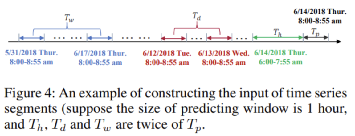
Three time series segments of length T_h, T_d, and T_w along the time axis are intercepted and used as the input of the recent, daily-period, weekly-period component respectively.

The three components have the same network structure and each consist of several spatial-temporal blocks and a fully-connected layer.

Spatial-Temporal Attention

Spatial attention

In the spatial dimension, the traffic conditions of different locations have influence among each other and the mutual influence is highly dynamic.

Temporal attention

In the temporal dimension, there exist correlations between the traffic conditions in different time slices, and the correlations are also varying under different situations.

Spatial-Temporal Convolution

The spatial-temporal attention module let the network automatically pay relatively more attention on valuable information. The input adjusted by the attention mechanism is fed into the spatial-temporal convolution module. The spatial-temporal convolution module proposed here consists of a graph convolution in the spatial dimension, capturing spatial dependencies from neighbourhood and a convolution along the temporal dimension, exploiting temporal dependencies from nearby times.

Graph convolution in spatial dimension

Spectral graph theory extends the convolution operation from grid-based data to graph-structured data. In this study, the traffic network is represented as a graph, where each node's features are signals on the graph. To leverage the network's topology, graph convolutions based on spectral graph theory are applied at each time slice, processing these signals and exploiting spatial correlations. This spectral method transforms the graph into an algebraic form to analyse its topological attributes, such as connectivity.

Convolution in temporal dimension

After the graph convolution operations having captured neighbouring information for each node on the graph in the spatial dimension, a standard convolution layer in the temporal dimension is further stacked to update the signal of a node by merging the information at the neighbouring time slice.

Multi-Component Fusion

It can be observed that the traffic flows at some areas have obvious peak periods in the morning, so the outputs of the daily-period and weekly-period components are more crucial. However, there are no distinct traffic cycle patterns in some other places, thus the daily-period and weeklyperiod components may be helpless. Consequently, when the outputs of different components are fused, the impacting weights of the three components for each node are different, and they should be learned from the historical data.

Experiments

Datasets

PeMSD4, PeMSD8

Baselines

HA, ARIMA, VAR, LSTM, GRU, STGCN, GLU-STGCN, GeoMAN

Metrics

MAE, RMSE

Results

• DIFFUSION CONVOLUTIONAL RECURRENT NEURAL NETWORK: DATA-DRIVEN TRAFFIC FORECASTING

Introduction

This paper proposes a model that uses the pair-wise spatial correlations between traffic sensors using a directed graph whose nodes are sensors and edge weights denote proximity between the sensor pairs measured by the road network distance. The dynamics of the traffic flow is viewed as a diffusion process and propose a diffusion convolution operation that captures spatial dependency. The full model architecture - Diffusion Convolutional Recurrent Neural Network integrates diffusion convolution, seq2seq architecture, and scheduled sampling.

Methodology

Spatial dependency modelling

Spatial dependency is modelled using a diffusion process which can capture the innate stochasticity of a traffic's dynamics. This is done by a random walk on the graph. Lemma 2.1 from Teng et al. (2016) is referenced:

The stationary distribution of the diffusion process can be represented as a weighted combination of infinite random walks on the graph, and be calculated in closed form

Temporal dynamics modelling

GRU is used to capture temporal characteristics.

For multi-step forecasting, seq2seq is employed, where both the encoder and decoder are RNNs with DCGRU. During training, historical time series is fed into the encoder and its final state is used to initialise the decoder. The decoder generates predictions given previous ground truth observations. Entire network:

Experiments

Datasets

METR-LA, PEMS-BAY

Baselines

HA, ARIMA, VAR, SVR, FNN, FC-LSTM

Results

That is all for today!

See you tomorrow :)