[Day 155] Reading more about 'historic' (used as baseline) models for spatio-temporal predictions using graphs
Hello :)
Today is Day 155!
A quick summary of today:
The updated graph with reference connections from Obisdian is:

Real-time Prediction of Taxi Demand Using Recurrent Neural Networks
Introduction
This paper proposes a real-time method for predicting taxi demands in different areas of a city. A big city is divided into smaller areas and during a pre-set period of time, the number of taxi requests in each area is aggregated. This way taxi data becomes a sequence and a LSTM is applied. LSTM is capable of learning long-term dependencies by utilising some gating mechanisms to store information. Therefore, it can for instance remember how many people have requested taxis to attend a concert and after a couple of hours use this information to predict that the same number of people will request taxis from the concert location to different areas. Simply learning the average to predict will not result in a very good model, so the paper adds Mixture Density Networks (MDN) on top of the LSTM. This way, instead of directly predicting a demand value, the output is a mixture distribution of the demand.
Mathematical model
GPS data encoding
A city is split into 153m x 153m area sizes. Then past taxi data is converted into week-long data sequences, which are the input to the LSTM.
RNNs

Taxi demand prediction model
Mixture density networks
MDNs can be used in prediction applications in which an output may have multiple possible outcomes. This paper's model outputs the parameters of a mixture model - the mean and variance of each Gaussian kernel and also mixing coefficient of each kernel which shows how probable the kernel is.
potential gold
LSTM-MDN sequence learning model


LSTM-MDN-Conditional model
In the LSTM-MDN model, the probability distribution of taxi demands in all areas are predicted at the same time-step. This means that prediction in each area is conditioned on all areas of all previous time-steps. However, the taxi demand in an area might not only be related to the past, but also to the taxi demands of other areas in current time-step. So instead of outputting a joint distribution for all areas in a single time step, the network predicts the conditional distribution of each area at a single time-step.


Results


Graph WaveNet for Deep Spatial-Temporal Graph Modeling
Introduction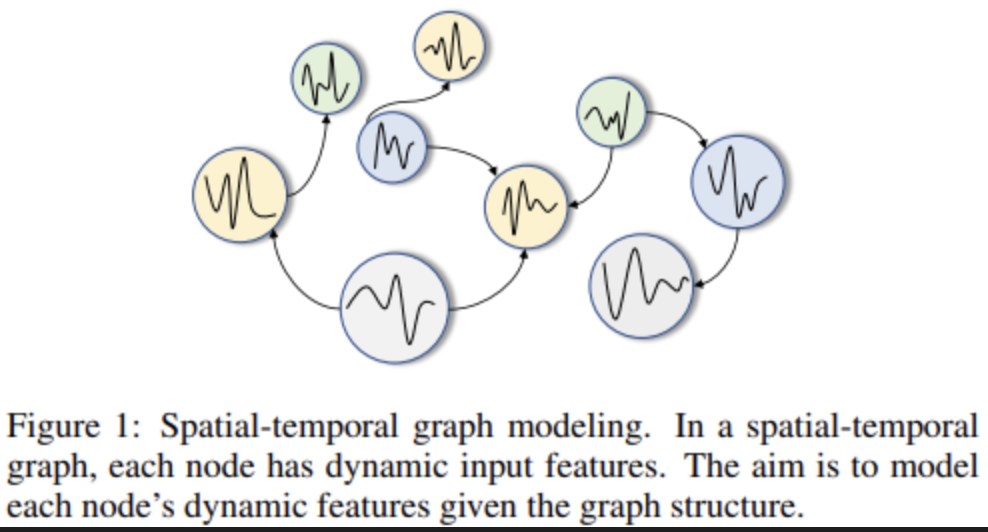
A basic assumption behind spatial-temporal graph modelling is that a node’s future information is conditioned on its historical information as well as its neighbours’ historical information. Paper contributions:
- A self-adaptive adjacency matrix is constructed to preserve hidden spatial dependencies. This matrix automatically uncovers unseen graph structures from the data without prior knowledge. Experiments show that this method improves results when spatial dependencies exist but are not provided.
- Additionally, an effective and efficient framework is presented to capture spatial-temporal dependencies simultaneously. The core idea is to combine the proposed graph convolution with dilated causal convolution, allowing each graph convolution layer to address the spatial dependencies of nodes’ information extracted by the dilated causal convolution layers at different granular levels.
Methodology
Problem definition
Given a graph G and S historical time steps, predict the next T time steps.
Graph convolution layer
The paper proposes a novel self-adaptive adjacency matrix, which does not require any prior knowledge and is learned end-to-end through SGD. This way the model can learn hidden spatial dependencies by itself.
Temporal convolution layer
Dilated causal convolution are used as TCN to capture temporal trends. Dilated causal convolution networks expand the receptive field exponentially by increasing layer depth. Unlike RNN-based methods, these networks can effectively manage long-range sequences in a non-recursive manner, enabling parallel computation and reducing the risk of gradient explosion. Dilated causal convolution maintains temporal causal order by padding inputs with zeros, ensuring that predictions at the current time step only use historical data. As a variant of standard 1D convolution, the dilated causal convolution operation skips values at regular intervals while sliding over the inputs.


Experiments
Datasets
METR-LA and PEMS-BAY
Baseline models
ARIMA, FC-LSTM, WaveNet, DCRNN, GGRU, STGCN
Results

The impact of the self-adaptive adjacency matrix is examined through experiments conducted with Graph WaveNet, utilizing five different adjacency matrix configurations. Results indicate that even in the absence of prior graph structural knowledge, the adaptive-only model outperforms the forward-only model in terms of mean MAE. The forward-backward-adaptive model demonstrates the lowest scores across all evaluation metrics, suggesting that incorporating the self-adaptive matrix enhances model performance when graph structural information is provided. Further analysis of the learned matrix reveals variations in node influence, with nodes near intersections exerting more influence compared to those along single roads.

GMAN: A Graph Multi-Attention Network for Traffic Prediction
Introduction
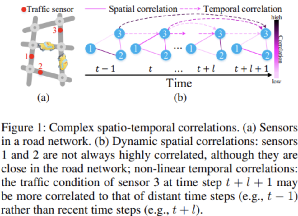
Complex spatio-temporal correlations
- The correlations of traffic conditions of a particular road change over time. It is difficult to pick out relevant sensors' data that will be useful to predict a target sensor's traffic conditions in the long-term.
- Non-linear temporal correlations. In cases of accidents, conditions may change suddenly. It is difficult to create an adaptive model to such non-linear temporal correlations.
Sensitivity to error propagation
- Small errors in each time step stack onto each other and can end up as big problems in a future step.
To that end, Graph Multi-Attention Network (GMAN) is proposed to predict traffic conditions on a road network graph over some time steps ahead. GMAN can be applied to any numerical traffic data, but this paper concentrates on traffic volue and traffic speed.
Related work
Traffic prediction
Popular historical approaches: LSTM, ARIMA, SVR, KNN, CNN, GCN.
Deep learning on graphs
Attention mechanism
Graph multi-attention network

Spatio-temporal embedding
Using node2vec, vertices are converted into vectors that preserve the graph structure information.
For temporal embedding, each time step is encoded into a vector.
The above are combined as a spatio-temporal embedding (2b).
ST-Attention block
Includes spatial attention, temporal attention and gated fusion.
Spatial attention


When the number of vertices (sensors) gets large, the time and memory consumption is large. To tackle this issue group spatial attention is proposed which contains intra-group spatial attention and inter-group spatial attention.
Temporal attention

The traffic condition at time t is correlated with times before t as well, and this correlation can vary over time (it is non-linear). To measure the relationship between different time steps both traffic features and times are considered.
Gated fusion
The traffic condition of a road at a certain time step is correlated with both its previous values and other roads’ traffic conditions. As seen in picture 2c, spatial and temporal embeddings are fused together.
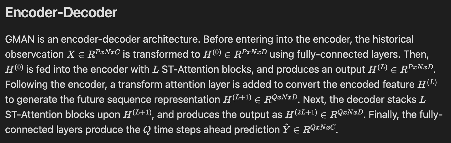
Transformer attention
To mitigate error propagation across different prediction time steps in a long-term forecast, a transformer attention layer between the encoder and decoder is introduced. This layer captures the direct relationships between each future time step and all historical time steps, transforming the encoded traffic features to produce future representations, which serve as the decoder's input.

Experiments
Datasets

Metrics
MAE, RMSE, MAPE
Hyperparametres
Baselines
ARIMA, SVR, FNN, FC-LSTM, STGCN, DCRNN, GraphWaveNet
Results

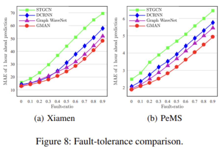
The real-time values of traffic conditions may be missing partially, due to sensor malfunction, packet losses during data transmission, etc. To evaluate the fault-tolerance ability, a fraction of historical observations is randomly dropped to make 1 hour ahead predictions
Effect of each component

DNN-Based Prediction Model for Spatio-Temporal Data
Introduction
Different from text and image data, ST data has two unique attributes: 1) spatial properties, which consists of a geographical hierarchy and distance, and 2) temporal properties, which consists of closeness, period and trend.
Models
Definitions
Region
- a city is partitioned into an M x N grid map based on the longitude and latitude where a grid represents a region
Measurement
- crowd flows are used. For a grid that likes at the m-th row and n-th column, two types of crowd flows at the k-th timestamp - in-flow and out-flow
DeepST

Evaluation
Datasets


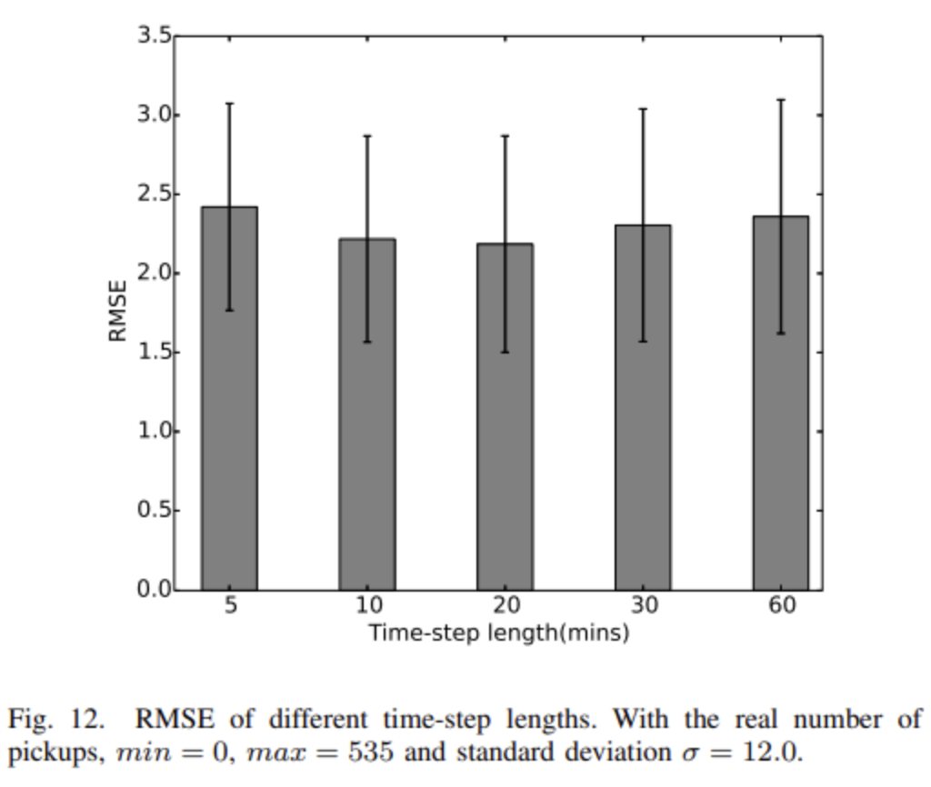
Evaluation metric
RMSE
Results


That is all for today!
See you tomorrow :)

