[Day 150] Learning more about taxi OD matrix prediction + Scottish dataset update
Hello :)
Today is Day 150!
A quick summary of today:- read a few more papers about taxi demand and Origin-Destination matrix prediction using Graph Neural Networks
- added more audio clips to the Scottish (Glaswegian) dataset
Obisdian makes this nice graphs of papers referencing each other.

First paper is Modeling Long- and Short-Term Temporal Patterns with Deep Neural Networks
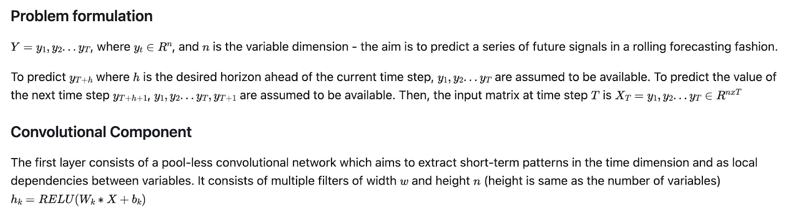
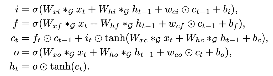
(some will be pictures because I am yet to find a better way to share the math notations)
Introduction
Multivariate time series forecasting can learn traffic jam patterns ahead of time. However, a common challenge is capturing dynamic dependencies across multiple variables. For example the traffic on a highway can experience two patterns - daily (morning vs evening traffic) and weekly (weekday vs weekend). If a model is not able to handle complex data, then time-series forecasting is not feasible. To this end, the authors propose the usage of deep neural networks (RNN and CNN), and in particular - Long- and Short-term Time-series Network (LSTNet).
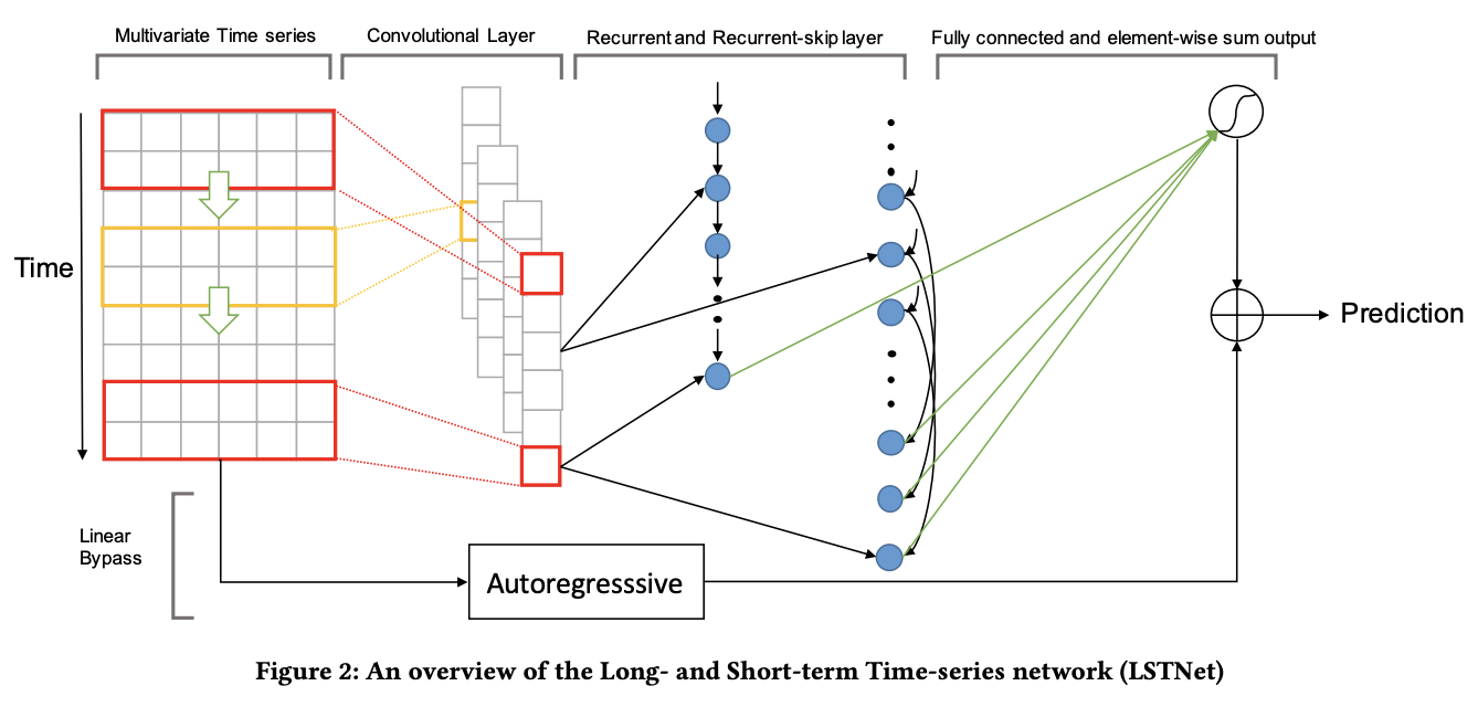
It combines the strength of convolutions to discover local dependency patterns among multi-dimensional input variables and the recurrent layer which can capture complex long-term dependencies. It also uses a 'Recurrent-skip', which helps with capturing long-term patterns and makes optimisation easier. Finally, a traditional autoregresive linear model is used side-by-side with the non-linear deep learning model for more robustness when the data has violate scale changing.
Related Background
Autoregressive integrated moving average (ARIMA) is one of the most famous univariate time series models due to its statistical properties and Box-Jenkis methodology. ARIMA models are adaptive, flexible and subsume other models like autoregression (AR), moving average (MA) and Autoregressive Moving Average (ARMA). However none of the above are used in high dimensional multivariate time series forecasting due to high computational costs.
Vector autoregression (VAR), on the other hand, is one of the most used models in multivariate time series due to its simplicity. However, the model capacity grows linearly over the temporal window size, and quadratically over the number of variables which results in VAR models overfitting easily.
Linear methods are often preferred for multivariate time series forecasting due to the availability of high-quality off-the-shelf solvers in the machine learning community. However, similar to VAR models, these linear approaches may struggle to capture the intricate non-linear relationships present in multivariate signals. Consequently, while linear models offer efficiency, they may sacrifice performance when faced with complex non-linear dynamics.
Another type of method is the non-parametric Gaussian Processes (GP). However, it comes at a high price in terms of computational complexity.
Methodology
The above output is fed through the Recurrent component and Recurrent-skip component in parallel. The Recurrent component is a GRU and the output is the hidden state at each time step.
Autoregressive Component
The autoregressive (AR) component is integrated into the LSTNet architecture to counteract the scale insensitivity of neural network models like CNNs and RNNs, particularly when faced with non-linear and non-periodic changes in input signals. AR models excel at capturing linear trends and dependencies in time series data, providing a complementary approach to the non-linear components of LSTNet. By combining both AR and non-linear components, LSTNet can effectively capture both linear and non-linear patterns in the data, enhancing forecasting accuracy.
Evaluation
Methods for comparison
AR, LRidge, LSVR, TRMF, GP, VAR-MLP, RNN-GRU, LSTNet-skip, LSTNet-Attn
Data

Results

2nd paper: Structured Sequence Modeling with Graph Convolutional Recurrent Networks
Introduction
Graph Convolutional Recurrent Network (GCRN) is a generalization of RNNs to data structured as a graph.
Combinations of CNN and RNN models have been explored for videos and images, where CNN is used for visual feature extraction followed by a RNN for sequence learning.
This paper leverages the above to propose the GCRN model for predicting time-varying graph-based data, and at the core is merging CNN for graph-structured data and RNN to identify simultaneously meaningful spatial structures and dynamic patterns.

Proposed GCRN Models
Model 1
Stacking a graph CNN for feature extraction, and an LSTM for sequence learning

Comparison between models


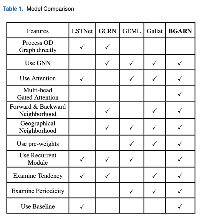
3rd paper: A Baselined Gated Attention Recurrent Network for Request Prediction in Ridesharing
Introduction
Related work
Majority of work uses GNNs over CNNs to capture the non-Euclidean nature of the space and a LSTM to capture the temporal dynamics. Typically, the request data is preprocessed into a (OD) grid map, then neighbour data is aggregated (for spatial features), such as Semantic Neighborhood and haversine distance. These grids from the OD Graph form a new feature graph, where one directed edge represents the propagation tendency of the features from one grid to another. With the support of Graph Neural Networks (GNNs), the feature propagation among the nodes is performed, and the output grid matrix specifies the extracted request forwarding pattern. A time series of these grid matrices is then pushed into a recurrent module like Long Short-Term Memory (LSTM) to integrate the temporal features, such as tendency and periodicity (also referred to as trend and period). Finally, the output spatial-temporal features are translated back to a new OD Graph to predict the future request flow.
[[GCRN]] does not use spatial features, instead it processes the OD matrix directly as a spatial feature. However, this increases the initial feature dimensions. This problem is solved by [[Gallat]] and [[GEML]] by specifying semantic and geographical neighbourhoods. Gallat further splits the Semantic neighbourhood into forward and backward which shows that grids have different importance as an origin and destination. Furthermore, the above two models also use pre-weighted functions that take the contributions of different neighbours into account.
Simple GNNs do not account of for different importance along different edges and this is important in this OD problem because the connections between grids vary due to spatial dynamics. To this end, GAT was proposed which leverages edge weights using Attention.
From a time point of view, there are papers which replaced the LSTM with GRU for reduced computation cost, others with a Transformer for capturing long-term temporal dynamics.


Spatial Attention Layer
Originially introduced in GEML and Gallat, below are the definitions for spatial analysis.
- Forward neighbourhood
- Backward neighbourhood
- Geographical neighbourhood
Temporal Recurrent Layer

This layer uses the previously produced spatial-temporal embedding matrix for two tasks: demand prediction for the next time slot, and the OD matrix for the next time slot. Baseline models: HA and AR (Auto-Regressive) Using the baseline results and the prediction results from the spatial-temporal embedding matrix, the Transferring Layer obtains the final prediction outputs. Equations for task:

where Aggr(.) specifies the tuning approach which can be sum, weighted sum or multiplication (by default).
Dataset and Results


As for the Scottish dataset
I got home and I preprocessed the ~150 clips (postprocess count of audio clips that my Scottish collaborator had sent me). And now we have a total of ~16 minutes of audio clips in Glaswegian. I also tried to finetune microsoft T5 again but my colab ran out of free credits. So tomorrow while working, I will use my PC.

That is all for today!
See you tomorrow :)

