[Day 149] Learning about the Origin-Destination Matrix Prediction problem in passenger prediction tasks
Hello :)
Today is Day 149!
A quick summary of today:- back in the lab and read 2 papers about Origin-Destination Matrix Prediction via Graphs
I decided to start using obsidian to take notes and it is amazing. It is also good practice writing math using latex. Also for some reason I cannot copy paste the math formulas, so some of the text below is in pictures so that the formula (math notation) can be included for clarity. I need to figure out a way to better share these notes.
Paper 1: Gallat - Passenger Mobility Prediction via Representation Learning for Dynamic Directed and Weighted Graph (DDW)
Introduction
At first, studies concentrated on passenger demand as a function of starting location and time period. However, this failed to account for the passengers' destination. This was tackled by the definition of Origin-Destination Matrix prediction problems, where there are different time slots with their own OD matrix describing travel demand from region i to region j. Based on this ODMP, Graph Neural Networks have emerged as the go-to solution because of their ability to capture complex relationships and compared to previously applied CNNs, generalise to non-Euclidean graph topologies.
Definitions
Methodology
- pre-weighted functions - helps with the data sparsity. In addition to node semantic similarity, the obtained weights also incorporate real-time popularity of neighbour regions
Temporal Attention Layer
This layer can capture the sequential dependencies among embeddings and generate spatiotemporal representation for predicting the passenger demand in the next time slot. A naive approach to this would be to gather information from P most recent and consecutive DDW graphs. This might not work that well since in reality, a graph at time T will have similarity with graphs in close time slots, and if the time difference is too big this will introduce noise into the learned graph representation. To improve on that, the paper uses P historical DDW graphs form the same time slow of each day.
Transferring Attention Layer
Focusing on the next time slot, we can predict passenger demands between regions. Initially a vector with outbound passenger demands at the next time slot T+1 is created. Then it is distributed to different regions using a probability distribution that indicates the likelihood of a passenger trip from one region to every other region in the next time slow.
Experiment
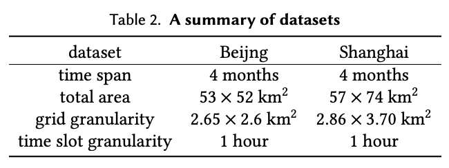
Dataset
Baseline models
History Average (HA), LSTNet, GCRN, GEML
Results
0,3,5 are thresholds for demand. I.e. threshold 0 includes all regions, threshold 3 includes regions where there is at least 3 passenger demands
Paper 2: GEML - Origin-Destination Matrix Prediction via Graph Convolution. A New Perspective of Passenger Demand Modeling
Introduction
The ODPM problem is essential to solve for large taxi companies, as it will give information about customers' demands from one place to another. ODPM provides info about combinations of different origins and destinations, and the demand for each origin-destination combination. The target is to predict the number of orders from one place to another in a given time slot.
OD matrix construction
Methodology
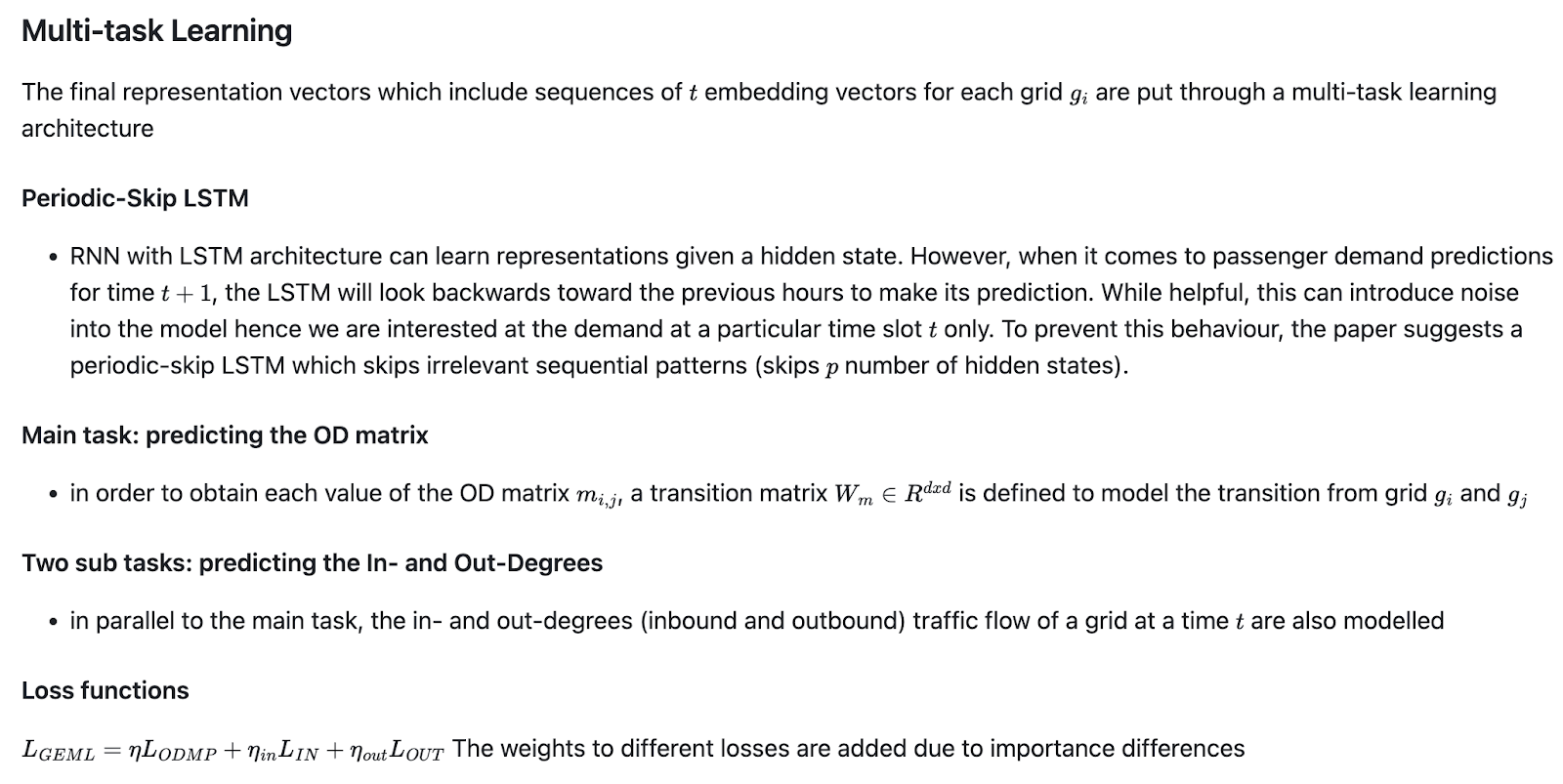
Grid-Embedding based Multi-task Learning (GEML)
OD matrices are extracted from mobility records of ride service providers. Then the grid embedding part of GEML learns the embedding vector for each grid through aggregating geographical and semantic neighbours information. Next, the vector representation is put through a multi-task neural network which learns the grid for the most recent time slot. Finally, the result is used to for a predicted OD matrix. In the authors' proposed model, both spatial information - using a neighbour-based grid embedding to learn each grid's representation by aggregating neighbour information, and temporal information - using the multi-task neural network that can learn dynamic trends of passenger movement over time, is captured.
Grid embedding
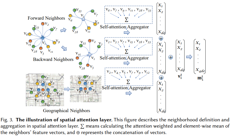
GCNs are limited when it comes to sparse graphs - which can happen in low demand areas. To tackle this, the authors propose two kinds of neighbourhoods for better neighbourhood aggregation - geographical and semantic neighbours. This achieves to measure the closeness between a grid and its neighbours and in addition, the traffic flow's semantic strength between origin and destination.
Evaluation
Compared with History Average (HA), LSTM, LSTNet, GCRN
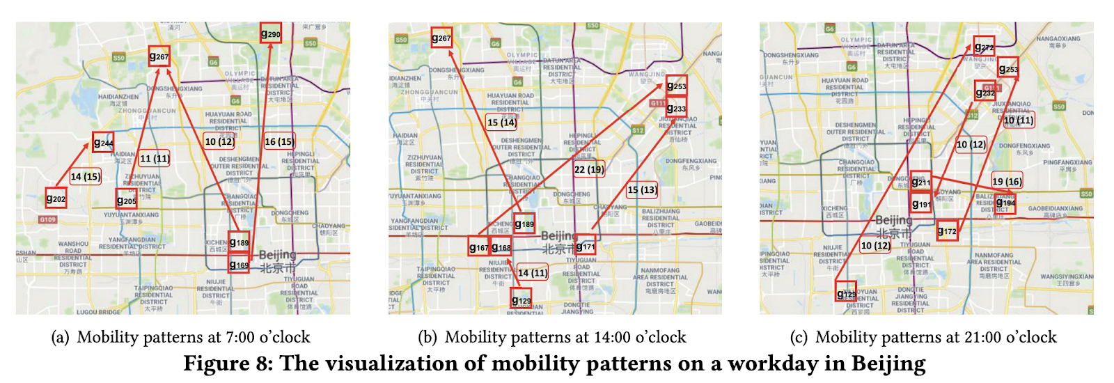
Visualisation
(a) Morning mobility: people leave home and go to different destinations. g202, g205, g189, g169 are residential areas, while g267, g290 are software parks
(b) Post-lunch mobility: there are still many passengers going to work/entertainment venues.
(c) Evening mobility: there are people going home, but also going to entertainment venues
That is all for today!
See you tomorrow :)


