[Day 125] MLx Fundamentals Day 2: Causal representation learning, optimization

 Hello :)
Today is Day 125!

A quick summary of today:

• listened to day 2 lectures on causality and optimization of MLx Fundamentals
• learned a bit of STATA

The schedule was:

The recording of the lectures was released about 30 mins ago, so going over it will be my task for tomorrow. 

The 1st lecture from Professor Kun Zhang from CMU was more specifically about causal representation learning. 

For example finding hidden variables. 

Here if we look at just the relationship between cholesterol and exercise (right graph) we can see they have a positive relationship. Which is quite weird, and when we incorporate age into the picture, we can see the actual negative relationship. 

In this case there are treatment A and B for kidney stones, and if we just look at the overall, without accounting for stone size, we might conclude that B is better. But if we incorporate stone size into the picture, A is better in both cases. if we understand the problem well, there is no paradox because we know that Both is wrong because there is a hidden variable - in this case size of the stone

The 2nd lecture by Professor Chi Jin from Princeton University was amazing. I got a ton of resources and even though it was math heavy - the explanations were very clear and the TAs helped a lot in the lecture's slack channel. I will take notes and share on a later day when the recording gets uploaded.

Actually from this lecture I got very nice extra material to dive deeper into optimization after I rewatch and take notes of his lecture last night:

• Professors Chi Jin's lectures on Optimization in Princeton from Spring 2021
• Lectures on Convex Optimization (Yurii Nesterov 2018)
• Convex Optimization: Algorithms and Complexity (Sébastien Bubeck 2015)

The 3rd practical session on Optimization and DNN by Ziyan Wang from King's College London - as it was 2-3.30am for me in Korea I could not attend live but I went over the colab myself (I will need to rewatch later for any extra info that was shared), and below is a summary.

Part I of the practical session (Optimization)

For a simple model:

X = np.linspace(0, 1, 100)

y = 5 * X + 2

We see how the params converge over the epochs

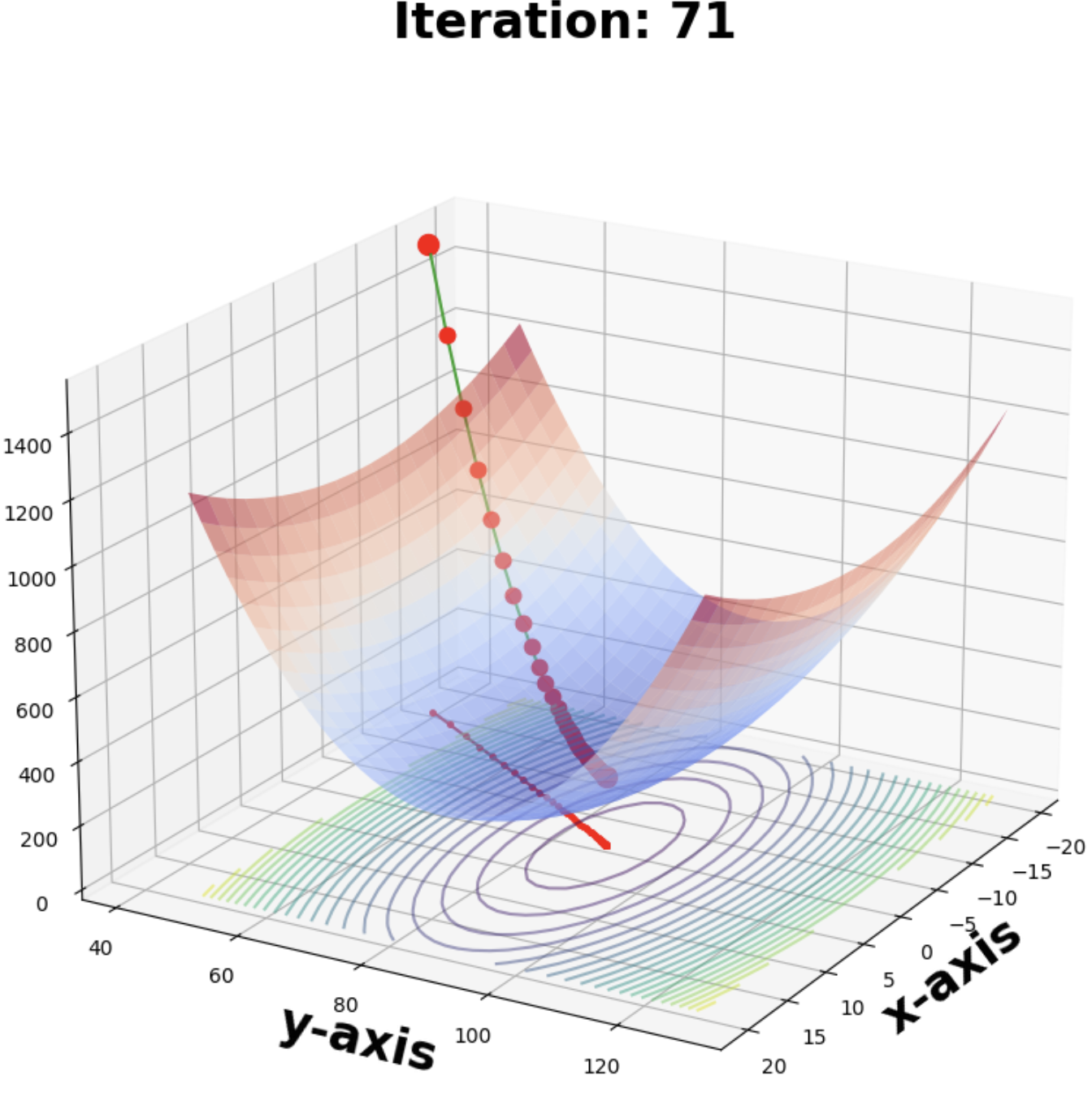
Then using scikit-learn's make_regression function we saw the loss function's surface

And how it moves through iterations

Here is a case with a smaller learning rate

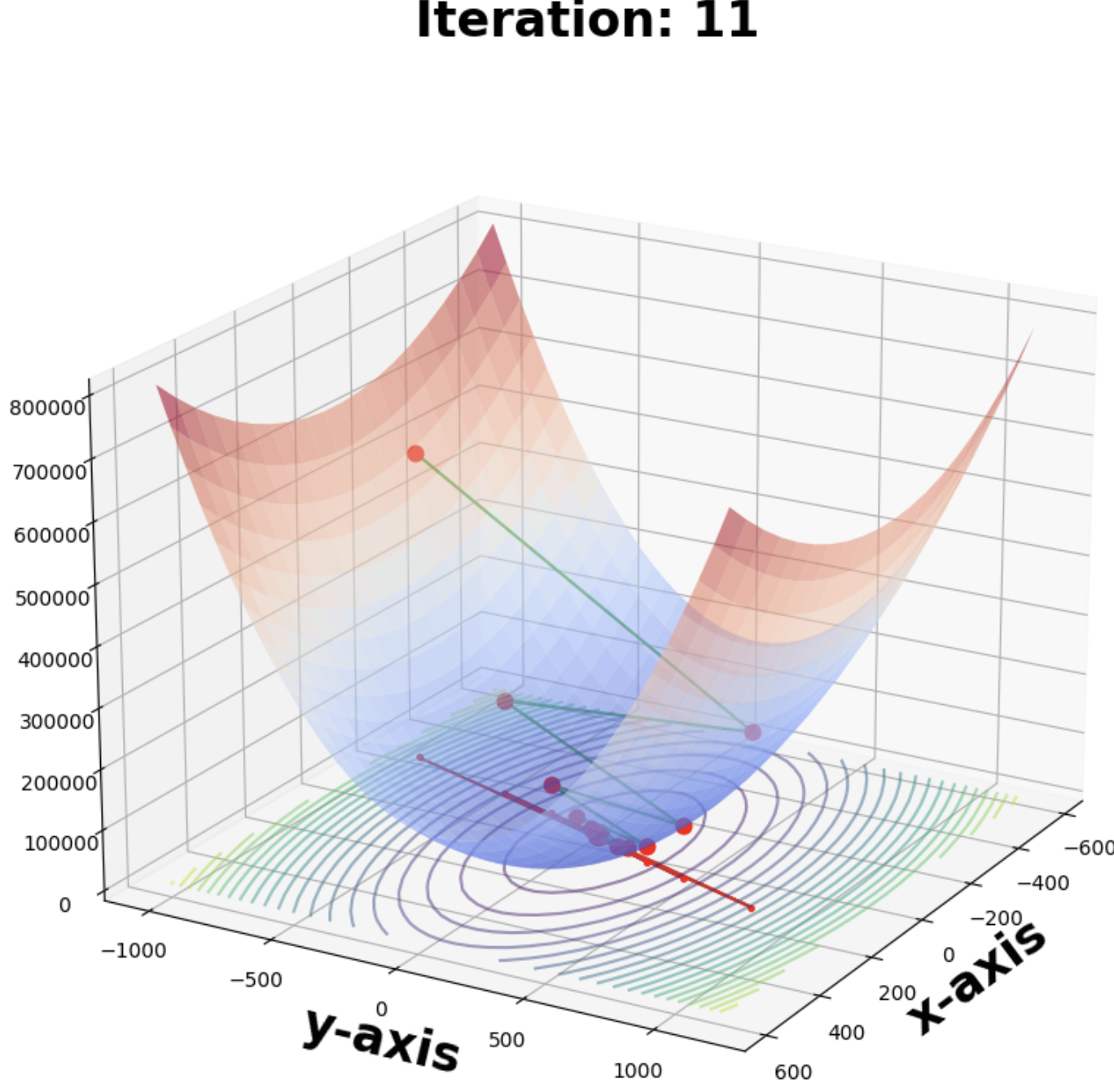
And a case where the lr is too big where the algorithm actually diverges (ending at the top)

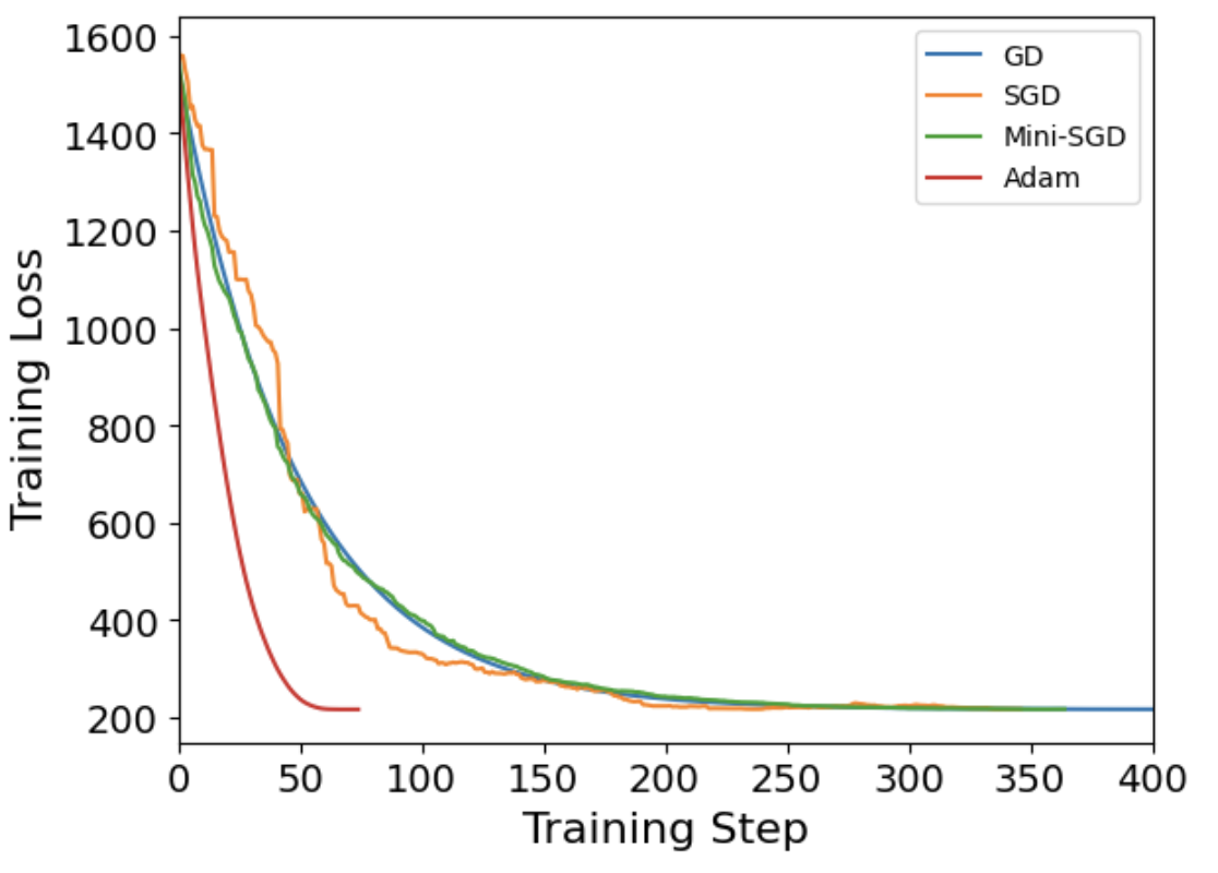
Finally we saw a comparison on the same loss surface of GD, SGD, mini-SGD and Adam (pictures are in the same order)

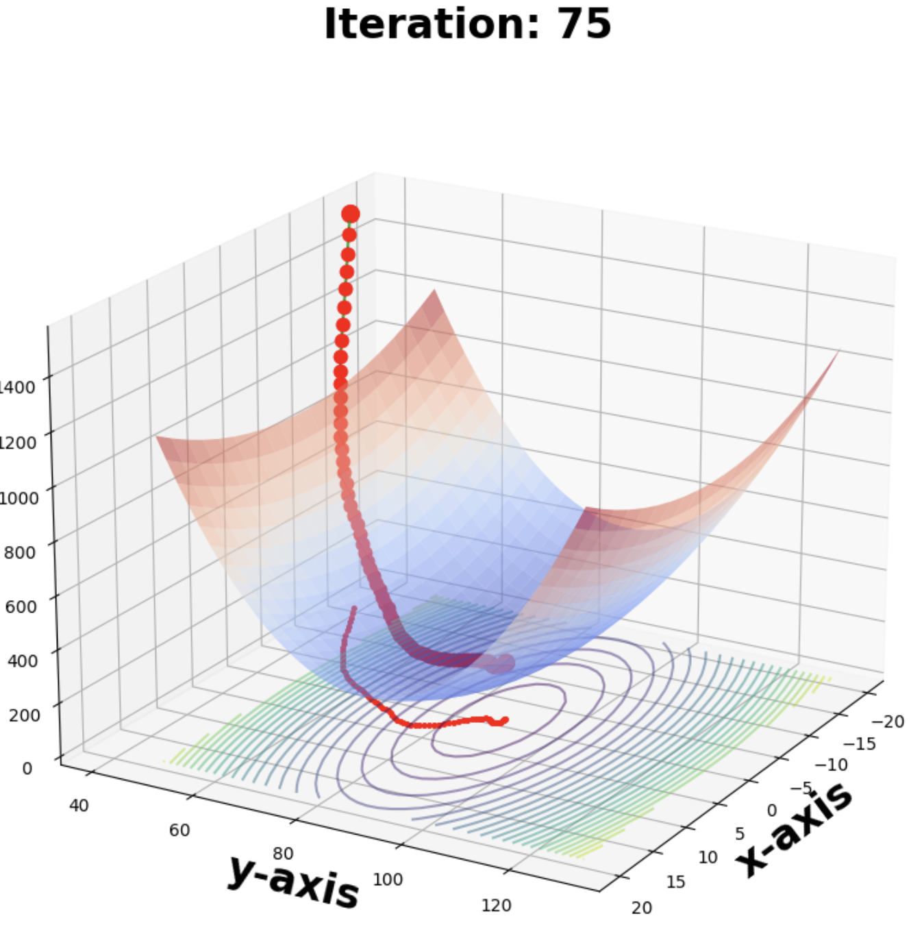
comparison

There was Part 2 as well, about building a simple CNN model to classify CIFAR images.

As for why I wrote that I learned a bit of STATA

For my girlfriend's class, she has to build some kind of linear model using data that she found online. We found some data about MPI (Multidimensional Poverty Index) from the University of Oxford, and I helped her with some data clearning and manipulation in python. There are probably functions like that in STATA as well, but she wanted to learn a bit of python. We dealt with some missing variables, got dummies for categorical variables, and then I joined her to see how running a regression is stata looks like. We can use the `reg` and the 1st variable after is the y, and the one(s) after that are Xs. Also we ran some VIF (using `estat vif`) to explore multicollinearity. 

That is all for today!

See you tomorrow :)